A Simplified Approach to Backtesting Trading Strategies

This blog post focuses on a novel way to backtest trading strategies, aiming to reduce the chances of backtest overfitting. The technique uses statistical characteristics from historical data to generate synthetic datasets for testing.

The Issue of Backtest Overfitting

In the field of investment strategies, overfitting happens when a strategy performs well on historical data but poorly on new, unseen data. One common way to avoid this problem is by calibrating trading rules based on the stochastic process generating the data, rather than purely relying on historical simulations.

Understanding the Investment Strategy

Let's consider an investment strategy $S$ which invests in multiple opportunities. The value of each opportunity at any given time $t$ can be calculated as $m_i \times P_{i, t}$, and the profit/loss after $t$ transactions is represented as $\pi_{i, t} = m_i \times (P_{i, t} - P_{i, 0})$.

The strategy uses a standard trading rule for exiting an opportunity when either of the following conditions are met:

1. The profit crosses a pre-defined threshold $\bar{\pi}$.
2. The loss crosses a pre-defined threshold $\underline{\pi}$.

The trading rule is defined by these thresholds $\{ \underline{\pi}, \bar{\pi} \}$.

The goal is to find the optimal set of these thresholds, often denoted as $R^*$, that maximizes the Sharpe ratio, $SR_R$, defined as:

Defining Overfitting in Trading Rules

A trading rule is considered overfit if it is expected to perform worse than the median of alternative rules in out-of-sample data.

Algorithm to Find Optimal Trading Rules

The algorithm for finding optimal trading rules involves these steps:

1. Estimate the parameters $\{\sigma, \varphi\}$.

The rest of the algorithm will be discussed in the next section.

def optimal_trading_rule(
    sigma: float,
    phi: float
) -> Tuple[float, float]:

function optimal_trading_rule(
    sigma::Float64,
    phi::Float64
) -> Tuple{Float64, Float64}

View More: Python | Julia

These functionalities are available in both Python and Julia in the RiskLabAI library.

Using Synthetic Backtesting for Optimal Trading Rules in RiskLabAI

The RiskLabAI library offers a function for synthetic backtesting, which is useful for developing optimal trading rules without overfitting to historical data. This function can be implemented in both Python and Julia.

def syntheticBackTesting(
    forecast :float,
    halfLife :float,
    sigma :float,
    nIteration =1e5 :int,
    maximumHoldingPeriod=100 :int,
    profitTakingRange=np.linspace(.5,10,20) :np.array,
    stopLossRange=np.linspace(.5,10,20) :np.array,
    seed=0 :float
) ->np.matrix:

function Syntheticbacktesting(
    forecast ::Float64,
    halfLife ::Float64,
    σ ::Float64,
    maximumIteration =1e3 ::Int64,
    maximumHoldingPeriod = 100 ::Int64,
    profitTakingRange = LinRange(0.5,10,20) ::Array,
    stopLossRange = LinRange(0.5,10,20) ::Array ,
    seed = 0 ::Float64
) ::Matrix:

View More: Python | Julia

Functionality

The function operates on parameters like forecast prices, half-life of the model, and standard deviation. It then runs multiple iterations to identify optimal trading rules based on a combination of profit-taking and stop-loss ranges. The aim is to maximize the Sharpe ratio.

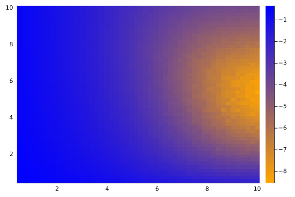
Experimental Results

The experiments suggest that there is a unique optimal trading rule that can be determined for a financial instrument whose price follows a discrete Ornstein-Uhlenbeck (O-U) process.

References

1. De Prado, M. L. (2018). Advances in financial machine learning. John Wiley & Sons.
2. De Prado, M. M. L. (2020). Machine learning for asset managers. Cambridge University Press.